May the Odds Be In Your Favour
Your Task
For each contestant of the Series 19 of UK Taskmater, generate probability distributions on their ranking in an episode.
For example, estimate the probability of Fatiha-El Ghorri placing 1st, 2nd, 3rd, 4th and 5th in an episode of Series 19.
A New Dawn, A New Dataset
With Series 19 well underway (at time of writing, Episode 8 “Science all your life” has just broadcasted), and a potential lag in the data being supplied to TdlM database1, it is time to take data matters into our own piano capable hands.
We are not completely abandoning the TdlM database, but for the purpose of the task in hand (it ideally is performed as the series broadcasts), it is useful to create, manage, and control our own dataset. This way we can ensure that the most recent episode data is available, and is of high quality.
Google Sheets
A Series 19 Google Sheets has been created by to track basic information on series of the information. Tabs include:
- Contestants: Information on the contestants, including their name, intials, URL to an image of them, and their seat number.
- Attempt-Tasks: Each contestants task attempt in each episode of the series. This is the most important dataset.
- MetaData: Data used for verification and quality purposes.
Data can be imported into R from Google Sheets via the package googlesheets4. For the purpose of our task in hand, only the Attempts-Tasks and Contestants are only required.
library(googlesheets4)
gs4_auth(email = "themedianduck@gmail.com")
gs_data_link <- "https://docs.google.com/spreadsheets/d/1DruoLL3X1HJAfUzE13_ZlAyXzshRvFHMCIVx9ncM6NI/edit?usp=sharing"

task_attempt_df <- range_read(gs_data_link, sheet = "Attempts-Tasks")

contestants_df <- range_read(gs_data_link, sheet = "Contestants")
A sample of the Attempts-Tasks tab can be found in Table 1.
| Series ID | Episode ID | Task ID | Task | Task Type | Contestant | Points |
|---|---|---|---|---|---|---|
| 19 | 1 | 1 | The object that most reminds you of school, in a good way | Prize | Fatiha El-Ghorri | 1 |
| 19 | 1 | 1 | The object that most reminds you of school, in a good way | Prize | Jason Mantzoukas | 5 |
| 19 | 1 | 1 | The object that most reminds you of school, in a good way | Prize | Mathew Baynton | 4 |
| 19 | 1 | 1 | The object that most reminds you of school, in a good way | Prize | Rosie Ramsey | 3 |
| 19 | 1 | 1 | The object that most reminds you of school, in a good way | Prize | Stevie Martin | 2 |
| 19 | 1 | 2 | Pour all the vinegar into the fish tank | Pre-Record | Fatiha El-Ghorri | 4 |
| 19 | 8 | 4 | Obey the autocue | Pre-Record | Stevie Martin | 4 |
| 19 | 8 | 5 | Play your people right | Live | Fatiha El-Ghorri | 1 |
| 19 | 8 | 5 | Play your people right | Live | Jason Mantzoukas | 2 |
| 19 | 8 | 5 | Play your people right | Live | Mathew Baynton | 4 |
| 19 | 8 | 5 | Play your people right | Live | Rosie Ramsey | 3 |
| 19 | 8 | 5 | Play your people right | Live | Stevie Martin | 5 |
The Observed Reality Timeline Approach (ORT)
A first approach, and most good starting point to estimate the probabilities is to base it off of the observed placement of each contestant at the end of each episode. From this, we can count the number of times a contestant has placed in a particular ranking, and normalise with respect to the number of episodes that have transpired so far. We refer to this as the observed reality timeline (ORT) method to estimate the probabilities.2 That is:
\[ \texttt{Probability of Fatiha placing 1st in an Episode} = \frac{\texttt{Number of time Fatiha has placed 1st}}{\texttt{Total Number of Episodes Fatiha has participated in.}} \]
and more generally,
\[ \texttt{Probability of Contestant $c$ placing $r$ in an Episode} = \frac{\texttt{Number of time Contestant $c$ has placed in $r^{\texttt{th}}$ position}}{\texttt{Total Number of Episodes Contestant $c$ has participated in.}} \tag{1} \] The ORT estimates are essentially the empirical proportions of a contestant ranking in that position.
Figure 1: Probability Distribution of Contestant Ranking Placement within in a Episode, based on the Observed Reality Timeline method.
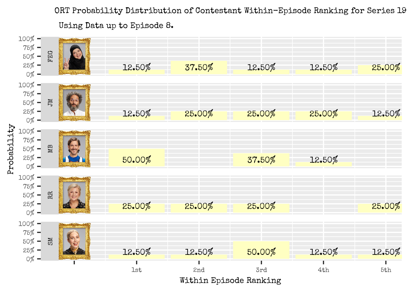
Figure 1 shows these estimated probabilities under the ORT approach using all data up to an including Episode 8 of Series 19. There are no major surprises in the results and insights generated. In particular:
- Matthew Baynton has a 50% probability of placing 1st in an episode, which makes sense since he has won 4 out of 8 episodes so far.
- He also has only placed 3rd or 4th in the remaining 4 episodes thus far, and has estimated probabilities of 37.50% and 12.50% respectively.
- As he has never placed 2nd or 5th so far in the series, he has an estimated probability of 0% for each of these placements respectively.
- For the other contestants, their probabilities are (unsurprisingly) in line with how they have been performing so far in the series:
- Fatiha is most likely to place 2nd with 37.50%, and 5th with 25%. The remaining placements are with equal probabilities of 12.50%.
- Jason is most likely to place 2nd, 3rd and 4th with 25%, and the remaining 12.50% either in 1st or 5th.
- Rosie has placed 1st, 2nd, 3rd and 5th an equal number of times across the 8 episodes, and thus her estimated probability is 25% on each. She has never placed 4th, and thus has an estimated probability of 0%.
- Stevie has placed 3rd 50% of the time and thus has an estimated probability of achieving this placement in an episode. Her remaining placement probabilities are 12.50%.
Do You Want Me To Stop the Clock?
We have a way of estimating probability distribution for a contestant’s placement in a episode! Job done, stop the clock.
One advantage of the ORT approach is the simplicity and intuitive nature of it. It is grounded in reality as it is based on contestant’s placement in each episode. Consequently, it is simple to calculate (low computational power) and can be conveyed easily to others.
Figure 2: Stop the clock Alex!
The Drawback of the Backdraw
However, one potential drawback of the ORT approach is that if a contestant has not ended up in a particular place for a episode, our probability estimate of this event occurring is 0%.
Whilst this is true from the observations we have, it is potentially misleading to assign a probability of 0% with such definitiveness. It could be that this event has not occurred yet (but is still probable and possible), or is an extremely rare event (extremely rare is not the same as impossible).
One consequence of this approach is that at the beginning of the series when data is limited, many of the probabilities will be 0% since we have not observed that particular (contestant, placement ranking) combination. Consequently, the ORT estimated probabilities are likely not representative of what could occur later in the series.
The Multiverse Approach (MV)
In the spirit of seeming hip, cool and aware of popular culture, it is time to introduce the concept of a multiverse, and how we can use this analogy to generate a distribution of probabilities which are more representative of all potential timelines and events.
The multiverse theory speculates that for every instance in which an action, decision or outcome is made, there is an alternative reality and timeline in which the alternative action, decision or outcome prevailed. For example,:
- We currently live in the timeline in which the US Taskmaster version was not a success.
- As a result, Little Alex Horne is still heavily involved in UK Taskmaster and writing the Horne Section TV Show.
- However, there is an alternate timeline where the US Taskmaster was a success. Who knows what consequences this could have reaped, but I would imagine:
- Little Alex Horne is less involved in the UK Taskmaster (he’s flying to the US frequently for US Taskmaster) and the quality of each UK series slowly decreases over time.
- As a result, we don’t get Series 19 of UK Taskmaster (the show has been cancelled before this), and the entertainment provided by the current cast.
In the context of Taskmaster and this task, the ORT is just one realisation of a particular timeline involving the series 19 cast in which a particular set of tasks were performed. There are potentially other timelines and alternate universes involving the Series 19 cast in which the contestants performed a different set of tasks, and the contestant placements are different. These alternative timeline and universes define the multiverse that we operate in.
We can use these alternative timelines and capture more potential outcomes, even if they have yet to be observed (or will ever be). It is these alternative timelines that will also help generate a probability distribution for contestant placement within an episode, which is more informative and potential outcomes of the series. We refer to this method of estimating probabilities as the MultiVerse Approach (MV).
What’s the Situation?
I’ll go into more detail in a later post of how these alternative timelines are simulated, and the generating the probability distribution of contestant placement within an episode. In short:
- The alternative timelines are generated through sampling and simulation based techniques.
- Sampling is performed (with replacement) on existing (contestant, task-attempt) data we have observed to date.
- Additional logic is then employed to group, re-rank and reassign points to contestants based on these samples.
- Once we have simulated these alternative timelines and outcomes, we can then estimate probabilities based on an equation similar to Equation (1).
- However under MV, we would be considering all alternative timelines we have simulated for both the numerator and denominator, and not just episodes that have brodcasted and observed.
In the statistical literature, this approach is based on concepts concerning sampling (in particular Bootstrapping), and Monte Carlo simulation methods.
The Customised Inhaler Gang
Figure 3: Probability Distribution of a Contestant Placement within an Episode, based on the MultiVerse method.
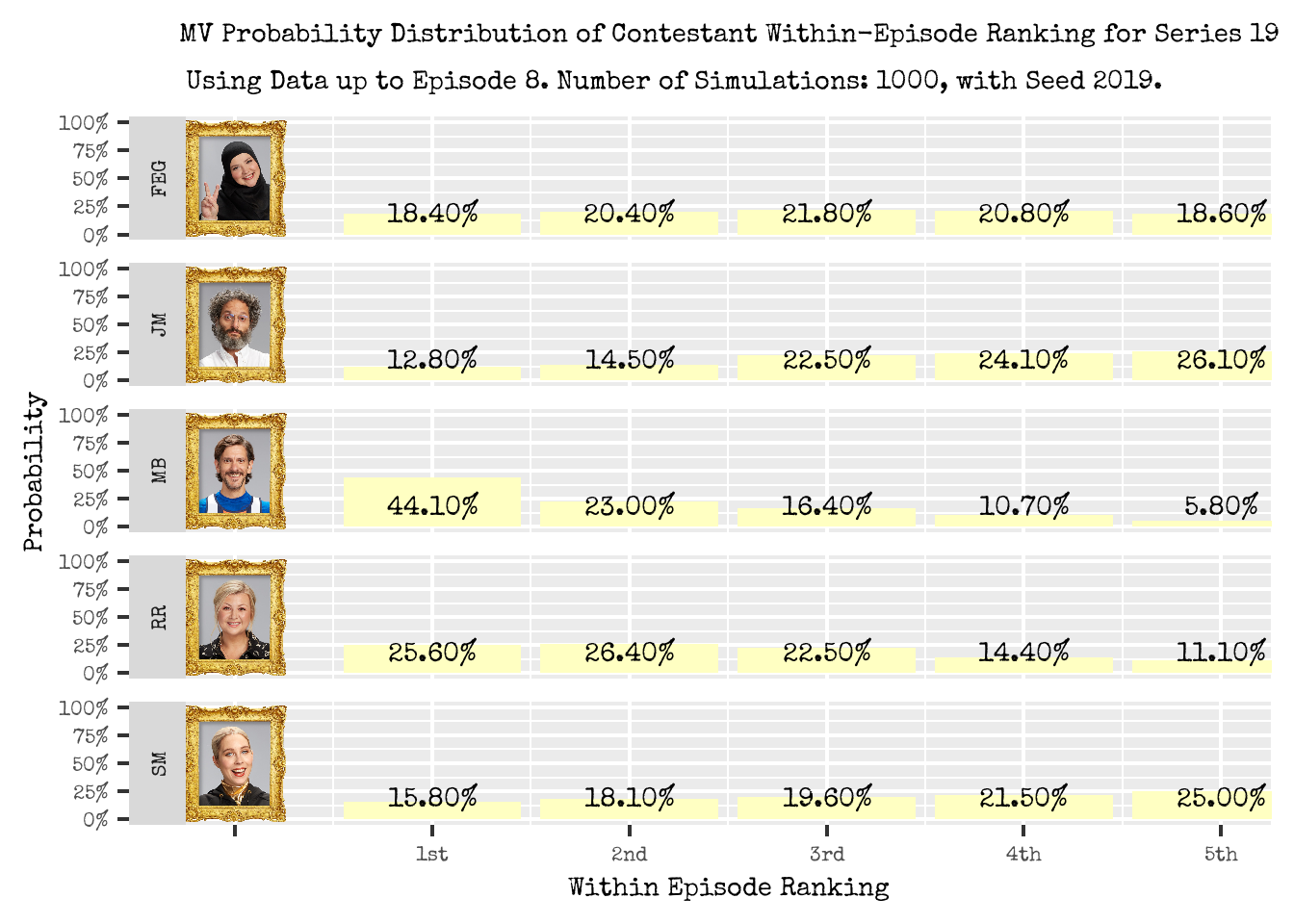
Figure 3 displays the probability distributions under the MultiVerse approach. It is based on using observed data up to and including episode 8 of Series 19, using 1000 simulations (that is 1000 alternative episodes were simulated), and random seed 2019 (based on 2025-05-01, the UK broadcast date of Episode 1 of Series 19)3.
- The MV probability distributions are “complete”: a non-zero probability is assigned to all contestant ranking combinations, even though these have not been realised.
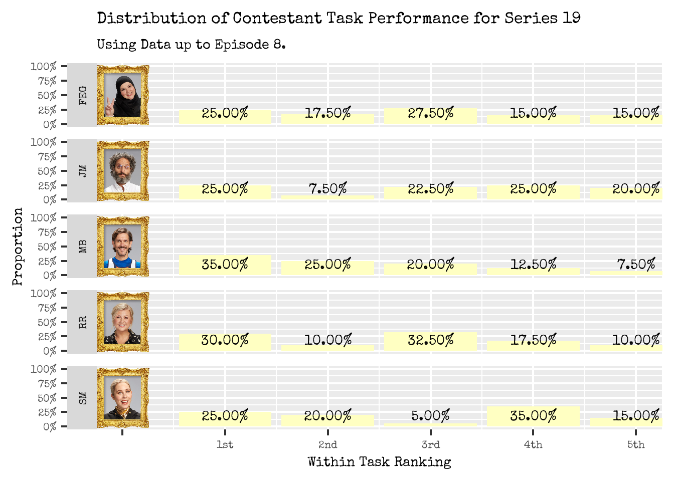
- The distributions for each contestant are peaked and skewed to how the contestants are ranking in the series overall (see Figure 4), and loosely to their general task performance (see Figure 5):
- For Fatiha, the distribution is symmetrical and peaked around 3rd place with a probability of 21.80%.
- She is currently placed 3rd in the series.
- For Jason, the distribution is skewed towards the lower rankings, with 5th place being the most probable outcome with 26.10%.
- He is currently placed 5th in the series.
- Matthew’s distribution is skewed towards the higher ranking position, with 1st place being the most probable outcome with 44.10%.
- He is currently placed 1st in the series.
- The probability of him ranking 5th in an episode is 5.80%.
- Rosie also has distribution skewedwed the higher ranking positions, although not as peaked as Matthew’s. Her most probable position is 2nd place with 26.40%, although her 1st place probability is a close second place with 25.60%.
- She is currently placed 2nd in the Series.
- Stevie has a similar distribution to Jason in that it is skewed towards the lower rankings. She is most likely to rank 5th in an episode with a probability of 25%.
- She is currently placed 4th in the series, although is only ahead of Jason (current 5th place), by 6 points.
- For Fatiha, the distribution is symmetrical and peaked around 3rd place with a probability of 21.80%.
- The MV distributions are noticeably different to the ORT distributions.
- This can be see as counter-intuitive in that it differs to the reality we have observed.
- However, it does make sense given that the MV methodology is based on a generalised performance of a contestant (captured through the simulation of many alternative timelines), whereas the ORT is based on a single realisation. This single realisation, could be representative of how a contestant performs in general, or a rarer extreme occurrence (they performed worse).
- The ORT distribution can also be misleading due to close finishes that may occur, or ties in placements.
- The generalised nature of how the MV distributions are generated also makes sense as to why it is aligned with the series ranking. The series ranking represents the general performance of a contestant across multiple episodes which have been broadcasted; the MV distributions represent the performance over episodes. These episodes have been simulated rather than broadcasted however.
Figure 4: Series Performance so far for Series 19.
Figure 5: Distribution of Contestant Task Performance.
Where Do we Go From Here?
One potential benefit of the MV approach is that we are likely able to produce distributions on series outcomes. For example:
- We are likely able to produce distributions on each contestants placement at the end of the series.
- For example, the probability of Fatiha finishing in 5th place at the end of series, or Jason winning the series (how improbable is it, or is it simply impossible?).
- We are able to also produce distributions on each contestants series points.
- For example, what is the probability of Jason scoring more than 140 points by the end of the series.
Figure 6: You have been warned of these plans…

However, the MV approach to estimate probability distributions of contestant ranking placements within an episode is by no means perfect. There are still some considerations and assumptions that needed to be expanded upon in the future. For example:
- Is 1000 alternate timelines (simulations) sufficient in obtaining the accurate, reliable probability distributions?
- Ideally, sufficient simulations have been performed such that the distribution does not drastically between randomness settings.
- A study of the number of simulations required to achieve a stable distribution is likely a topic for another post.
- The proposed MV method does not account for certain Taskmaster idiosyncrasies.
- For example, we do not distinguish between solo and team tasks. Nor do we account for “5 points to the winner, 0 for everyone else” instances, or Series 18’s Joker mechanism.
- Greater care and understanding of how ties should be handled. In particular, we do not consider tie breakers when two or more contestants having the highest number of points at the end of the episode. The winner of these tie breakers is officially deemed the winner of the episode (they get to take home the prizes), but does not affect the series points.
What Have We Learnt Today
We’ve learnt:
- We have a method to to estimate the probability distributions of each contestant’s ranking within a single episode.
- This method is a sampling, simulation based method which uses historical episode-contestant-task attempt which has already been observed. We effectively create alternate universes and timelines involving the Series 19 cast in which different task outcomes occurred.
- The estimated probability distributions are in line with the series rankings to date.
- The estimated probability distributions also capture realities and events which have not yet been observed.
- For example we can estimate the probability of Matthew Baynton ranking 5th in an episode, something that we have not observed so far.

It is still unclear what the service-level agreement is with this database in terms of when new data is expected to be available after transmission, fits our particular needs, and is of high quality (hopefully at least).↩︎
The ORT naming will make sense later in this post.↩︎
The notion of a random seed and the importance of setting it will become discussed in a subsequent post. It is to do with repeatability and controlling randomness.↩︎